Java in Flames. Profiler results
The integration with Java flames is conducted to evaluate the CPU overhead introduced by the perturbation instrumentation. I followed the instructions detailed in [1] to map Java stack frames to the linux-perf-tool.
The primary objective of this test is to compare CPU times between executions with and without perturbations. The initial results reveal a 1/4 ratio in execution times between the perturbed run and the unperturbed one. However, it’s important to note that the test subject for this experiment is the Quicksort algorithm. Therefore, for more comprehensive results, this test should be executed with more than one target.
Java in Flames
As [1] says: Java mixed-mode flame graphs provide a complete visualization of CPU usage and have just been made possible by a new JDK option: -XX:+PreserveFramePointer, this option become with a little time overhead in runtime, almost 3% more than the normal behaviour.
Without PreserveFramePointer the perf tool does not know the map between Java stack frames information and system ones and the resulting samples turn into a nonhuman understandable state.
Graph interpretation
From [1]
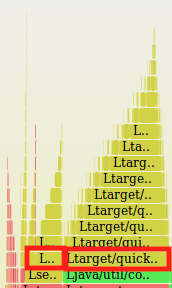
"If you are new to flame graphs: The y axis is stack depth, and the x axis spans the sample population. Each rectangle is a stack frame (a function), where the width shows how often it was present in the profile. The ordering from left to right is unimportant (the stacks are sorted alphabetically). In the previous example, color hue was used to highlight different code types: green for Java, yellow for C++, and red for system. Color intensity was simply randomized to differentiate frames (other color schemes are possible)."
"You can read the flame graph from the bottom up, which follows the flow of code from parent to child functions. Another way is top down, as the top edge shows the function running on CPU, and beneath it is its ancestry. Focus on the widest functions, which were present in the profile the most. "
Profiling run
The profiling execution has been made over the Quicksort pilot algorithm, sampling with a 500Hz frequency in a 120 seconds window, resulting in more than 72 000 samples, watching out to record the access registration step and the beginning of space exploration.
Instrumentation workflow
We follow the general proposed algorithm to make a perturbation space exploration in [2] to implement it on Java language.
1
2
3
4
5
6
7
8
9
10
11
12
13
14
15
for each input i in I do
    Rref = runWithoutPerturbation(prog, i)
    for perturbation point pp in prog do
        for j = 0, to Rref[pp, i] do
            o = runWithPerturbationAt(prog, model, i, pp, j)
            if exception is thrown then
                exc[pp] = exc[pp] + 1
            else if oracle.assert(i, o) then
                s[pp] = s[pp] + 1
            else
                ob[pp] = ob[pp] + 1
            end if
        end for
    end for
end for
Our Java code instrumentation
1
2
3
4
5
6
7
8
9
10
11
12
13
14
15
16
17
18
19
20
21
22
23
24
25
26
27
28
29
30
31
32
33
34
35
36
37
38
39
40
41
42
43
44
 1. while(inputProvider.canNext()){
 2.   Tin input = inputProvider.getIn();

 3.   Tout expected = provider.get(inputProvider.copy(input));

 4.   executeWithoutPerturbation(callback, inputProvider.copy(input));

 5.   Map<IPerturbationPoint, Integer> accessCount = engine.getAccessCount();
 6.   for(IPerturbationPoint pp: pps) {
 7.       pp.getRercods().clear();
 8.       pp.reset();
 9.   }

 10.  for(IPerturbationPoint pp: pps){

 11.       for(int i = 0; i < accessCount.get(pp); i++) {
 12.           pp.setTime(0);

 13.            int perturbAt = i;

 14.           Callable<Tout> callable = () -> executePerturbation(pp, StaticUtils.serviceProvider.getModel(), callback, inputProvider.copy(input), perturbAt);
 15.          try {
 16.               service.submit(callable);
 17.
 18.               Future<Tout> future = service.poll(engine.getExecutionTimeout(), TimeUnit.MILLISECONDS);
 19.               Tout result  = future.get();
 20.
 21.               if (result != null && checker.getExpected(result, expected))
 22.                   summaries.get(pp).successCount++;
 23.               else
 24.                   summaries.get(pp).wrongCount++;

 25.           } catch (Exception e) {
 26.               pp.reset(StaticUtils.serviceProvider.getModel());
 27.           }
 28.           pp.setTime(-2);
 29.       }


 30.  }

 31.   engine.resetAccessCount();

32.}
1
2
3
4
5
6
7
8
9
10
public <Tin, Tout> Tout executeWithoutPerturbation(ICallback<Tin, Tout> callback, Tin input) {

    StaticUtils.serviceProvider.setExecutionPolicy(IServiceProvider.ExectionPolicy.REGISTER_ACCESS);

    Tout result = callback.perturb(input);

    StaticUtils.serviceProvider.setExecutionPolicy(IServiceProvider.ExectionPolicy.PERTURBING);

    return result;
}
1
2
3
4
5
6
7
8
9
10
public <Tin, Tout> Tout executePerturbation(IPerturbationPoint pp, IPerturbationModel model, ICallback<Tin, Tout> callback, Tin input, int time) {

    pp.perturb(model, time);

    Tout result = callback.perturb(input);

    pp.reset(model);

    return result;
}
Sampling
The sampling had been made using the time window mentioned previously, counting the Java frame time presence in the CPU, due to this behaviour the graph only shows a part of the execution code profile. However, we can obtain an idea of the complete perturbation execution.
In this particular case, we can observe the most samples concentration over a central zone in the graph, matching with a perturbation complete call for a given input.
Running only one perturbation by Java execution exploration can be a better option to measure every perturbation point impact.
General Results

Analysis
The resulting graph shows a remarkable concentration over auxiliary method calls, even when the samples count are lowered than the main methods. In the particular case on this profiling, the most auxiliary calls match with checking the access to integers/boolean returning, this calls count the “timeline” of a perturbation access, like the algorithm proposed by [2] shows, even when the only positive answer is obtained in line 4 of the Java algorithm above.
Maybe separate the codes or clean the translation to exploration space from the access counting gets better results.
The resulting graph shows a 3/70 relation between the main perturbed method and the access to a pInt/pBool method. This measurable relation brings an idea about how perturbation access methods shake CPU running times.
Comparing perturbed execution and the none one.
The graph does not show a remarkable information about the non-perturbed execution. Non perturbed access only provide the expected result to compare with the perturbed execution following the [2] proposed algorithm. In other words, every perturbation point acts as an iterator count for the space exploration, then, for each access to it, we have a perturbed execution. We have a relation of 1 to more than 100 (in Quicksort case) between non-perturbed code execution and the perturbed one.
We move the line 3 to 13 in the Java code above to provide a comparison between the perturbed code and the none one. The main idea is to provide the profiler with more non-perturbed samples in the CPU (or the same access count in the exploration algorithm). The result is showing below.
In the previous image, we can see a presence of 2.18% of original non-perturbed code besides 9.02% of the perturbed one for a given input. This observation enforces the premise of that exists a CPU overhead in a perturbation instance.